The Rendering Equation

If you have ever looked at a rendered image and thought “That looks real,” what you are really seeing is a model for light behaving the way it does in the physical world. At the core of physically-based rendering techniques, is something known as the rendering equation.

You can think of it as the master recipe for realistic images. Put simply, it tells us:

The amount of light that leaves a point in a given direction is the sum of the light that point emits and the light it reflects from all other directions.

Actually coming up with an equation that describes this phenomenon turns out be pretty difficult. The challenge is that light does not take a simple path. It bounces, scatters, gets absorbed, and sometimes even comes from the objects themselves.

In 1986, the rendering equation was born, thanks to the work by David Immel et al. and James Kajiya.

Rendering Equation (Basic Form)

Yes, I agree, it does look rather intimidating, but I assure you it really is just fancy math notation for simple physical concepts. Let’s go ahead and unpack it.

The first term $L_o (\vec{x},\vec{\omega_o})$ is the amount of light that leaves a point $\vec{x}$ in a given direction $\vec{\omega_o}$, i.e. the solution to our rendering equation. It is the quantity that we are interested in finding.

In order to render a point we want to know what light leaves that point in the output direction, so for rendering an point in space on screen, we are interested in the quantity $L_o$ for that point.

Let’s quickly explain some of the common terms in the equation:

• $\vec{x}$ is the location of the point we want to render
• $\vec{n}$ is the normal vector of the surface located at position $\vec{x}$
• $\vec{\omega_o}$ is the output direction (for example, towards the camera)
• $\vec{\omega_i}$ is the input direction (for example, from the light source)

The next term $L_e (\vec{x},\vec{\omega_o})$ is the light component due to emissivity of the point. For example if the surface is a metal that is extremely hot and glowing, then the surface itself also becomes a source of light, which becomes a part of the light output $L_o$ from this point.

Now, we can finally talk about that big scary integral:

Don’t worry, I promise I’ll make it really simple to understand!

That integral can be summarized simply as just the average of all the incident light on that point which is reflected in the output direction.

The integral itself $\int_{\Omega} \cdot\cdot\cdot \; d\vec{\omega_i}$ is describing an integral over something called $\Omega$.

$\Omega$ is the hemisphere centered around our point of interest $\vec{x}$. Specifically, this integral is carried out for every single possible incident direction $\vec{\omega_i}$, such that $\Omega$ is the hemisphere that satisfies the condition $\vec{\omega_i} \cdot \vec{n} > 0$ for every possible value of $\vec{\omega_i}$.

If that doesn’t make sense, this visual should help:

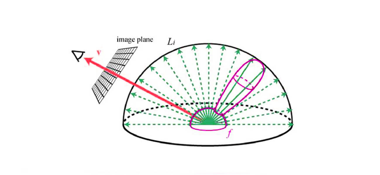
• The green arrows are different possible values for $\vec{\omega_i}$
• The red arrow is $\vec{\omega_o}$
• The black hemisphere is $\Omega$
• The location where all the green arrows originate from is $\vec{x}$ (i.e. the point we are trying to render)

The inner expression of the integral is made up of 3 parts.

First, there’s $L_i (\vec{x},\vec{\omega_o})$, which is the incoming light to point $\vec{x}$ from the direction $\vec{\omega_i}$

Second, we have this really weird function: $\textbf{BRDF} (\vec{x},\vec{\omega_i},\vec{\omega_o})$. This function is called the BRDF. Let us delve into what it is and what it does.

The BRDF

BRDF stands for Bi-directional Reflectance Distribution Function. Let’s break that down:

1. Bi-directional: It considers two directions as its input, $\vec{\omega_i}$ and $\vec{\omega_o}$
2. Reflectance: It models reflected light
3. Distribution: It describes a distribution of the reflected light
4. Function: It is a mathematical function that can be evaluated with different inputs

Putting all that together gives us our definition for what a BRDF is:

The BRDF is a function that describes how light arriving at a surface from one direction is reflected into another direction.

More specifically, it models the distribution of reflected light at a point on a surface given a certain incident direction.

A BRDF is made up of two components:

1. Diffuse reflection: Light that scatters evenly in many directions after hitting a surface, giving materials like chalk, fabric, or matte paint their soft, non-shiny look.
2. Specular reflection: Light that reflects more directly, creating highlights and shiny effects on materials like metal, glass, or ceramics.

The BRDF encodes surface material properties. Different surface materials will have different BRDFs. So essentially, the BRDF term is how the rendering equation makes a metallic surface look shiny, a wooden surface look rough, a glossy surface look smooth, etc.

Lambert’s Cosine Law

The last part of the inner expression in our integral $(\vec{\omega_i} \cdot \vec{n})$, is to account for Lambertian reflection.

A perfectly diffuse surface reflects light equally in all directions. However, the amount of light received depends on the angle of incidence: light coming in at a grazing angle spreads over a larger surface area, so less energy per unit area is available.

This property is modeled by Lambert’s cosine law and is calculated by taking the dot product of the incoming light with the normal direction. Since we are already multiplying by $L_i$ earlier, we only need to account for the value of the cosine factor, which we calculate as $(\vec{\omega_i} \cdot \vec{n})$.

Multiplying the incoming light $L_i$, the BRDF, and the Lambertian factor $(\vec{\omega_i} \cdot \vec{n})$ together, and averaging their output over all possible values of $\vec{\omega_i}$ gives us the solution to the integral.

Now, you know all of the parts of the rendering equation and what they mean!

Rendering Equation (Extended Form)

One thing you might have noticed is that in our rendering equation above we only account for surfaces that either absorb or reflect light. There is one additional case we have not account for, which is transmitted light.

Surfaces like glass transmit light directly through them, while materials like thin leaves cause light to undergo subsurface scattering, which also results in transmission.

Luckily the only thing we need to change in our rendering equation to fix this is the BRDF term.

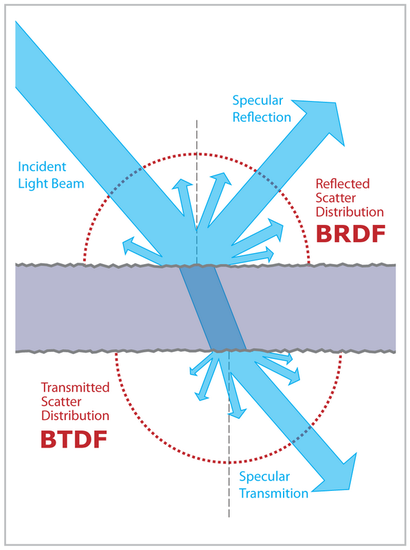
The BTDF

The BRDF, like the name suggests, only accounts for reflected light. We need a function that accounts for transmitted light. Conveniently it is called the Bi-directional Transmittance Distribution Function (BTDF).

The BTDF is a function that describes how light arriving at a surface from one direction is transmitted through it into another direction.

Another thing to note, is that when light is reflected, the incident direction and output direction are on the same side of the surface. However, when light is transmitted, the incident direction and output direction are on the opposite sides of the surface.

The BSDF

Now, we are interested in modeling light being absorbed, reflected, and transmitted through the surface so we can update our rendering equation. Currently, the BRDF only accounts for reflected light and the BTDF only accounts for transmitted light.

What we need is a combination of these two. That’s what the Bi-directional Scattering Distribution Function (BSDF) is. The BSDF is defined as:

• If $\vec{\omega_i}$ and $\vec{\omega_o}$ are on the same side of the surface, the BSDF is equal to the BRDF
• If $\vec{\omega_i}$ and $\vec{\omega_o}$ are on opposite sides of the surface, the BSDF is equal to the BTDF

Or in other words, the BSDF simply switches between being the BRDF or BTDF depending on directions of $\vec{\omega_i}$ and $\vec{\omega_o}$.

Final Rendering Equation

Now we can update our rendering equation to use the BSDF instead of the BRDF: